Thomas Schelling and Dr. Strangelove

January 31, 2014January 31, 2014 / Robert Sams / Leave a comment

An interview with Thomas Schelling and his role in the creation of one of my favorite movies, “Dr. Strangelove”. HKS reports,

Kubrick travelled to Cambridge to meet with Schelling and George. The three spent an afternoon wrestling with a considerable plot hole: when “Red Alert” was written in 1958, inter-continental ballistic missiles were not much of a consideration in a potential U.S.-Soviet showdown. But by 1962, ICBMs had made much of the book’s plot points impossible. The speed at which a missile strike could occur would offer no time for the plot to unfold. “We had a hard time getting a war started,” said Schelling.

Hence, the B52s?

Is Bitcoin volatility really in decline?

January 22, 2014January 22, 2014 / Robert Sams / 1 Comment

Eli Dourado has a great great blog that covers allot of issues concerning cryptocurrency, you should follow it if you don’t already. In a new post he reports that Bitcoin volatility has been trending down.

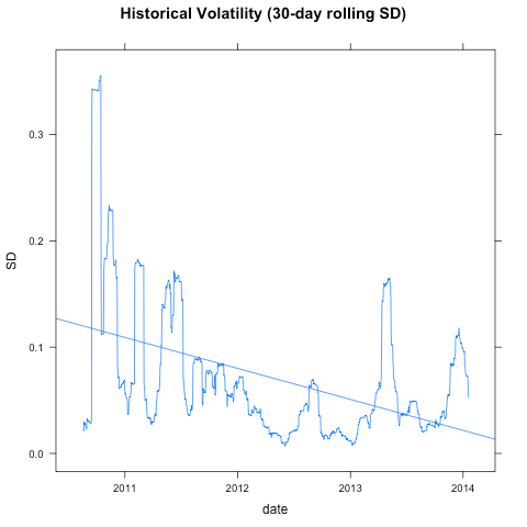
I calculated Bitcoin’s historical volatility using price data from
Mt. Gox (downloaded from Blockchain.info), which is the only
consistent source of pricing data over a long period. There is a clear
trend of falling volatility over time, albeit with some aberrations in
recent months. The trend is statistically significant: a univariate
OLS regression yields a t-score on the date variable of 15.

But the claim that “there is a clear trend of falling volatility over time” isn’t defensible at all. Before I explain why I don’t agree with with Eli, let me first replicate his analysis.

My OLS regression calibrates with Eli’s, so we’re on the same page:

                          Estimate   Std. Error   t value      Pr(>|t|)
(Intercept)           1.203775e-01 3.351178e-03  35.92095 3.489853e-194
seq(1, length(date)) -8.056651e-05 4.666856e-06 -17.26355  5.281210e-60

Putting that into English, the coefficient of the regression line is saying that volatility declines by about .00008 a day, or about 3 percentage points annually. Interpret that however you want.

And what is the daily volatility of BTC/USD?

    Min.  1st Qu.   Median     Mean  3rd Qu.     Max. 
0.007301 0.027890 0.048980 0.070220 0.082930 0.355300

About 5% per day. That’s pretty wild stuff, considering that the volatility of the S&P 500 is about 0.7% per day. But patience calls, one might say, for the trend line predicts that BTC/USD volatility is in decline.

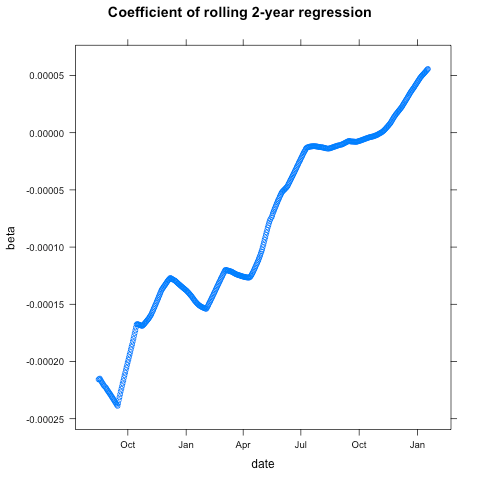
I don’t like using trend lines in analysing financial timeseries. Let me show you why. Here is a plot of the coefficient of the same regression, but on a rolling 2-year window.

This tells a very different story. The slope of that regression line flattens out and eventually changes sign, as the early months of BTC/USD trading fall out of the sample period. Here’s how the chart looks running that regression on the last two years of data.

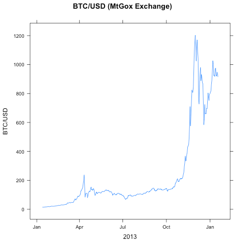
The trend reverses once the early stuff falls out of the sample. And there is good reason to exclude those early months from our analysis. Look at this chart of daily USD trade volume for those BTC/USD rates.

The price and volume series start around mid August 2010, but the volumes are really tiny for the first 8 months. And I mean tiny.. the median daily volume is about $3,300. Volumes get into the 5 and 6 digits after 13 April, 2011, when BTC/USD broke parity.

And before you say “that’s what we would expect, volatility to decline as volumes pick up”, look at those previous two charts. Volatility has been increasing as volume increases if you exclude the rinky dink period with sub-5-digit trading volumes.

Anyway, timeseries on thinly traded assets are notoriously unreliable. Those skyscraper patterns in the first chart are good hint that there’s some dodgy data in there. For example, Look at row 30:

                  date   price     volume         ror        vol
28 2010-09-13 19:15:05 0.06201   92.76696 -0.04598532 0.02973015
29 2010-09-14 19:15:05 0.06410 1293.53800  0.03370424 0.03019624
30 2010-09-15 19:15:05 0.17500 1035.82500  1.73010920 0.32375538
31 2010-09-16 19:15:05 0.06190   51.31510 -0.64628571 0.34284369
32 2010-09-17 19:15:05 0.06090  252.73500 -0.01615509 0.34271839

On September 15, 2010 we see a 173% daily return, followed by a -65% return the following day when the price basically returned to levels it was trading at on the 14th. Bad data point? Probably, but with these tiny volumes, does the question even matter.. this part of the series is junk.

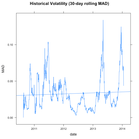
One way of handling these issues is to prefer a more robust estimator of volatility, like Mean Absolute Deviation (this is a common practice in trading systems research). So let’s re-run the OLS we started off with–including the rinky dink period–but this time using 30-day rolling MAD instead of SD.

Bummer, the trend disappears. Let’s look at it another way. A plot of daily returns is always a good visual check. (I stripped out those two dodgy data points we looked at above.)

You can clearly see that the largest two one-day declines happened within the last 12-months. In fact, 4 of the 5 the largest one-day losses happened in 2013, and those were multi-million dollar volume days.

           date   price   volume      ror      vol      mad
968  2013-04-12  83.664 34740413 -0.47654 0.136859 0.075185
967  2013-04-11 159.830 38009457 -0.32722 0.097551 0.069511
973  2013-04-17  79.942 25542665 -0.27551 0.154853 0.086190
1201 2013-12-07 767.777 83625810 -0.26372 0.108006 0.091285
84   2010-11-08   0.370    34758 -0.26000 0.227176 0.064088

And the 5 largest gains? All over two and a half years ago.

          date price    volume     ror     vol      mad
169 2011-02-01  0.95   70422.8 0.90000 0.17375 0.041508
69  2010-10-24  0.19    2612.9 0.74296 0.17274 0.018748
83  2010-11-07  0.50   44081.4 0.72413 0.22559 0.067911
296 2011-06-08 31.91 3238531.0 0.67418 0.17172 0.073743
257 2011-04-30  4.15  349701.7 0.53702 0.13500 0.048596

Now, I wonder, what charts the FX guys at Coinbase are looking at…

A quick look at Bitcoin transaction volume

January 19, 2014January 19, 2014 / Robert Sams / 11 Comments

A common rationale for owning Bitcoin is that its logarithmic money supply makes it a good store-of-value (SOV). Like precious metals or rare paintings stored in Swiss vaults, the scarcity of those coins will ensure that they at least keep their value.

By itself, this argument is hopelessly naive, as there is nothing scarce about a cryptocurrency with a fixed terminal money supply; anyone can (and a great many have) fork Bitcoin and create another such currency, so the total supply of such coins is potentially unlimited. But it could be replied that there are powerful network effects here, that the demand for digital SOV will coordinate around just one or two “crypto gold” stocks. In a previous post I’ve argued that the continuous hashing costs required to make the p2p secure would indeed imply such a network effect, but that the inability of log coin supply to finance these hashing costs out of seigniorage after the money supply stops growing casts doubts about the sustainability of this spontaneous digital gold enterprise.

A more sophisticated defence of Bitcoin’s valuation goes like this. Bitcoin is great SOV not just because of its limited supply and those hashing cost network effects. It’s a great SOV because in future more and more people will use it as a medium-of-exchange (MOE). As the volume of bitcoin transactions increases, so will the demand to hold bitcoin balances for the purpose of making transactions in goods and services. But a total of only 21 million bitcoins will ever be produced, so the price of a bitcoin must reflect the ratio of expected future MOE money demand to 21 million. The price of Bitcoin, one might argue, is the market’s prediction of the long-term growth rate of bitcoin transaction demand.

So let’s set aside the theoretical objection to this thesis and look at it empirically. Is there evidence of transaction growth to date that would rationalise Bitcoin’s valuation if we extrapolate recent tx growth?

Here are the daily transaction volumes and BTC/USD fx volumes aggregated from the main exchanges.

Just eyeballing this chart, it looks to me like there is very little transaction growth except for the period at the end of the first and fourth quarters, when there were dramatic revaluations in the exchange rate. And the explanation that leaps to my mind for those spikes in tx volume is that it’s coming from the settlement of fx trades for buy-and-hold positions in bitcoin, and a good deal of Chinese evasion of capital controls via CNY –> BTC –> USD, GBP, EUR..

But a more bullish story could be told. The revaluation of Bitcoin might have had a large wealth effect, with early Bitcoin adopters spending some of their increasingly dear hoard on weed and alpaca socks, and the revaluation was itself due in large part to newcomers buying bitcoin for the purpose of buying stuff with it.

Transactions on the blockchain that are settling an fx trade should be excluded from our calculation of bitcoin transaction growth. For every buy, there is a sell, so these transactions cannot represent new transaction demand by definition.

The data series used in these charts come from blockchain.info, and unfortunately, it only has fx volume for BTC/USD. Ideally, we’d want the volume figures for BTC vs EUR, GBP, CNY, JPY, and others so that we could add them all up and subtract total fx volume from the transaction series to get a truer picture of underlying transaction growth. If anyone can point me to where I can get those data easily, I’ll run the analysis.

Until then, here are monthly Bitcoin total transaction and BTC/USD trade month-on-month volume growth figures (in USD).

 yearmm     tx     fx
 201301  0.554  1.105
 201302  0.620  0.673
 201303  1.304  2.188
 201304  1.765  3.349
 201305 -0.388 -0.580
 201306 -0.318 -0.521
 201307  0.265 -0.183
 201308 -0.161 -0.323
 201309  0.112 -0.109
 201310  0.681  1.196
 201311  3.847  4.150
 201312 -0.015  0.207

Average Monthly Growth (2013)
   tx    fx 
0.413 0.418

These data are not conclusive. You could argue that the roughly 40% monthly tx growth is impressive evidence of underlying transaction growth. Or, you could interpret the roughly identical growth rates of tx and fx volume, and their high monthly correlation, as evidence that most of the tx growth is due to fx settlements. We need a complete fx volume series to disambiguate the data. When we do that, my bets are that monthly tx growth is under 20%.

The Marginal Cost of Cryptocurrency

January 15, 2014January 16, 2014 / Robert Sams / 46 Comments

I would count myself in the camp who believe that cryptocurrencies could do to finance what TCP/IP did to communications. Yet I also believe that Bitcoin and most of its current variations suffer from a fatal economic design flaw that will not survive the evolution of cryptocurrencies. That flaw is logarithmic money supply growth, and in this post I will explain why it is flawed. My argument is a microeconomic analysis of cryptocurrency and has nothing to do with the much debated “deflationary bias”. As far as I am aware, the argument in this post has not been made before.

In a recent post Tyler Cowen adapts an old chestnut of the money literature to cryptocurrencies. Cowen’s argument is based on some false assumptions, but it has the virtue of starting from the right microeconomic principles, so it’s an excellent point of departure.

Once the market becomes contestable, it seems the price of the
dominant cryptocurrency is set at about $50, or the marketing costs
faced by its potential competitors. And so are the available rents on
the supply-side exhausted.

There is thus a new theorem: the value of WitCoin should, in
equilibrium, be equal to the marketing costs of its potential
competitors.

In defence of the dominant cryptocurrency, Bitcoin, one might accept this argument yet object to its pessimistic conclusions by pointing out that Cowen is ignoring powerful network externalities. After all, coins residing on different blockchains are not fungible with one another. Cowen seems to treat these things as if they’re near substitutes, but maybe it’s a Visa/Mastercard sort-of-thing.

I want to dismiss this objection right away. We should be sceptical of ambitious claims about the network externalities of any one cryptocurrency. The network externalities of established fiat currencies are, of course, enormous, but this is largely due to their having a medium-of-account (MOA) function (to say nothing of legal tender and taxation), as well as a medium-of-exchange (MOE) function. Transactions settled in a cryptocurrency consult the exchange rate at the time of settlement and therefore piggy-back off the numeraire of an established fiat currency. Cryptocurrencies are not MOA, they are MOE only.

And given the near-frictionless fx between cryptocurrencies themselves, it’s not difficult to imagine a payment front-end for routine payees like on-line retailers that accepts a wide range currencies as MOE. And multi-coin wallet software for payers is a no-brainer.

So, for the sake of argument, I’m going to assume that the network externalities of any given cryptocurrency are close to zero. On Cowen’s analysis, this would imply that the marginal cost of cryptocurrency is near-zero. And this means:

Marginal cost of supply for the market as a whole is perhaps the
(mostly) fixed cost of setting up a new cryptocurrency-generating
firm, which issues blocks of cryptocurrency, and that we can think of
as roughly constant as the total supply of cryptocurrency expands
through further entry. In any case this issue deserves further
consideration.

This is a long-time objection to the workability of competitive, privately issued fiat currencies. The cost structure of their production cannot be rationalised with their value. A market of competing fiat currencies with “stable” purchasing power will generate too much seigniorage to their issuers, inviting more competition until the purchasing power of these media rationalise their cost of production.

If we can’t lean on the economics of network externalities, what’s wrong with this argument?

The marginal cost of new coins is the cost of hashing a block

First of all, Cowen speaks of a “cryptocurrency-generating firm” that issues “blocks of cryptocurrency”. The idea here seems to be that the marginal costs of creating a crypto coin are close to zero (it’s just data after all), most costs being the fixed costs of setting up the cryptocurrency system.

But this has things the wrong way round. Creating a new crypto currency is as easy has forking the Bitcoin source code, hacking it, and throwing the fork up on a code repo. Fixed costs are practically zero. Marginal costs, however, equal the electricity costs (and amortised hardware costs) of solving a new block of transactions, as each new block contains a mining award for the peer whose hashing finds a solution to the system’s hash problem. This is how new coins are created.

Mining in equilibrium

To compensate a peer for the costs of doing this costly hashing work, he is allowed to pay himself a certain number of new coins in a special coinbase tx each time he solves the hash problem on a block. But the protocol ensures that the expected value of this mining award is offset by the cost of the requisite kilowatt hours needed to do the hashing. There are no issuers here “collecting rents”; it’s as if the seigniorage is sacrificed to the entropy gods.

Miners (the peers who choose to do the hashing) will work on new blocks only when the expected value of the mining award exceeds the cost of electricity required to run the hashing hardware. There are no restrictions of entry to mining, and the equilibrating mechanism is the protocol’s hashing difficulty. If the coin’s exchange value increases, making mining profitable at current difficulty, more miners will join the hashing effort and because of this, after 2016 blocks the protocol will adjust the difficulty upward making expected value of mining = costs of mining again. The same process works in reverse in the scenario where exchange value decreases. In the creation of crypto coins, MC = MP.

(It should be noted that this is a stochastic rather than deterministic equilibrium, as the difficulty resets approximately every two weeks. Furthermore, the miner is paying for electricity today for an award he will get at some point in future, so it’s really more of a case of MC = E[MP]. But these details are not relevant to the conclusions we want to draw in this post, so I’ll continue to speak as if the marginal cost of making new coins equals the exchange value of coin at any given point in time.)

Why isn’t it obvious that MC = MP?

There are two properties of hash-based proof-of-work that obscure these microeconomics. The first is the multi-factored economics of mining difficulty. Improvements in specialised hashing hardware increase mining difficulty but do not increase its cost. (These improvements should eventually converge to a Moore’s Law function of time when the mining rig manufacturers exhaust all of the low-hanging fruit and run into the same photolithography constraints faced by Intel, etc.) The efficiencies merely result in a higher hashing difficulty, a sort of digital Red Queen Effect.

Similarly, increases (decreases) in the price of electricity will decrease (increase) the difficulty without changing the costs of mining. (It should also be noted that mining will gravitate towards regions like Iceland where it is cold and electricity is relatively cheap.) The only variable that does change the cost of mining is the exchange value of the currency itself.

And this is the other barrier to realising that MC = MP. In Bitcoin and most of the alt-coins, money supply is a logarithmic function of time. As money supply growth is deterministic, changes in money demand are reflected in the exchange value of the coin, raising or lowering the cost of producing the next coinbase as the protocol adjusts the difficulty up or down in response to the entry or exit of hashing power. So the exchange value of the mining award determines the marginal costs rather than the other way round. An economist might find that pretty weird, but that is how it works.

Network security and the crypto money demand function

It costs nothing to fork Bitcoin, hack the source, and create your very own alt-coin. But by itself, such a system is broken and has no bearing whatsoever on the economics of working cryptocurrencies. To make your alt-coin a working system, a sufficiently diverse group of miners must burn some costly kilowatt hours mining each block of transactions. Someone has gotta spend some capital to keep the lights on.

And the more kilowatt hours burned, the better, as the demand for a given cryptocurrency is a function of that system’s hashing costs (among other things, of course). The reason this is so has to do with the integrity of the most recent blocks on the distributed tx ledger, the blockchain. The amount of capital collectively burned hashing fixes the capital outlay required of an attacker to obtain enough hashing power to have a meaningful chance of orchestrating a successful double-spend attack on the system.

A double-spend is an event whereby the payee sees his payment N blocks deep and decides to deliver the goods or services to the payer, only to have this transaction subsequently not acknowledged by the network. Payments in cryptocurrency are irreversible, but double-spends are possible, and in economic terms they have the same effect that fraudulent chargebacks have in conventional payment systems like Visa or Paypal. The mitigation of this risk is valuable, and the more capital burned up hashing a crypto currency’s network, the lower the expected frequency of successful double-spend attacks.

Given that such events undermine confidence in the currency and drive its exchange value down (harming all holders, not just the victims of a double-spend), it should be axiomatic that a cryptocurrency’s hash rate is an argument of its money demand function.

This is also why it doesn’t make sense to speak of new cryptocurrencies expanding the aggregate crypto money supply without limit (or limited only by the fixed costs of creating one). What matters is how the aggregate hashing power, which is scarce, gets distributed over the set of extant cryptocurrencies. The obove reasoning predicts that hashing power will not spread itself arbitrarily thinly, keeping MC well-above 0. (The distribution currently looks more like a power law.)

Who pays to keep the lights on?

From the perspective of mitigating double-spend risk, the more capital that is burned hashing the better because the frequency of double-spend attacks is inversely related to the amount of capital burned. But the marginal benefits of hashing are at some point diminishing and the cost of hashing is linear, so for the end-user of a cryptocurrency, there is some level of hashing that is optimal.

In our argument above for why MC = MP, we made a simplification in saying that the mining award consisted entirely of coinbase. In fact, it consists of coinbase plus tx fees. In a protocol like Bitcoin’s where money growth is logarithmic, most of the early hashing costs are paid for out of new money supply, but as time goes on, tx fees become a greater and greater proportion of the mining award (currently, tx fees are about 1/3rd of Bitcoin’s mining award).

Now here we do see a genuine network externality. Imagine that all hashing costs are paid out of tx fees (as will eventually be the case with Bitcoin). There will be a natural tendency for demand for crypto MOE to gravitate towards the system with a higher tx volume, as it will have lower fees per-transaction for a given level of hashing.

Now imagine that we have a range of cryptocurrencies along a spectrum. On one end of the spectrum is the logarithmic money supply protocol–we’ll call these “log coins”. On the other end of the spectrum is a protocol with perfectly elastic money supply–we’ll call these “growth coins”. Growth coins have a non-deterministic money growth rule, an algorithm that enlarges the coinbase just enough to offset any increase in money demand, so the exchange value is roughly stable as long as money demand is not in decline. (In a future post, we will outline a protocol that can actually implement something approximating this.)

Where can we expect demand for MOE to gravitate along this spectrum of cryptocurrencies? This is where the logarithmic money growth rule hits the skids. At the margin, seigniorage for the log coins is eaten up by hashing costs, but as money demand outpaces the (rapidly declining) growth rate of money supply, the exchange value of the currency increases and existing coin holders are the recipients of the seigniorage on all of the existing, revalued coin.

Growth coins, by contrast, generate most of the seigniorage in the form of a larger coinbase rather than revalued coin, meaning that most of the seigniorage is spent on hashing. The result is lower tx fees for the those who use growth coins as a MOE.

Given that tx fees will be shared between payer and payee, it’s hard to see how magic network economics will maintain the dominance of the log coins in the long run. Money demand coming from the transaction motive will gravitate towards the MOE with the lowest tx costs.

Free-riding not gold buying

The scenario gets worse when we relax the monetarist assumptions (latent in the above analysis) of stable money velocity and demand proportional to tx growth. You don’t have to be a Keynesian to see how a large quantity of Bitcoin balances are held for speculative reasons. The high level of coin dormancy in the Bitcoin blockchain is as conclusive empirical evidence of this as there can be.

Bitcoin, therefore, has a free rider problem, whereby speculative coin balances, which benefit from the system’s costly hashing rate are effectively subsidised by those who use bitcoins primarily as a MOE. These speculative balances repay the favour by adding a toxic amount of exchange rate volatility, providing yet another reason for the transaction motive to run away from log coin MOE. As time goes on and the coinbase declines, this inequitable arrangement only gets worse.

Optimal cryptocurrency

As long as the growth rate of a growth coin’s money demand is sufficient to generate enough seigniorage in coinbase to cover the hashing rate demanded of its MOE users, transactions in growth coin are basically free. Some negligible fee will likely be required to deter DoS attacks (which has the interesting consequence of putting the goals of Adam Back’s Hashcash back into the cryptomoney that appropriated its designs), and its hard to see how one who wishes to hold crypto coin balances for the purpose of actually making transactions would prefer a log coin over a growth coin.

So maybe here is a new theorem: the value of a cryptocurrency will converge to its optimal level of hashing costs?

Fiat money via hash-based proof-of-work breaks new ground and we need to give the concept the attention and analysis it deserves. After all, we can dispense with the barbarous relic of logarithmic money supply and keep the good bits.

cryptonomics

the economics of crypto-markets

Month: January 2014